Heat Pump and Organic Rankine Cycles

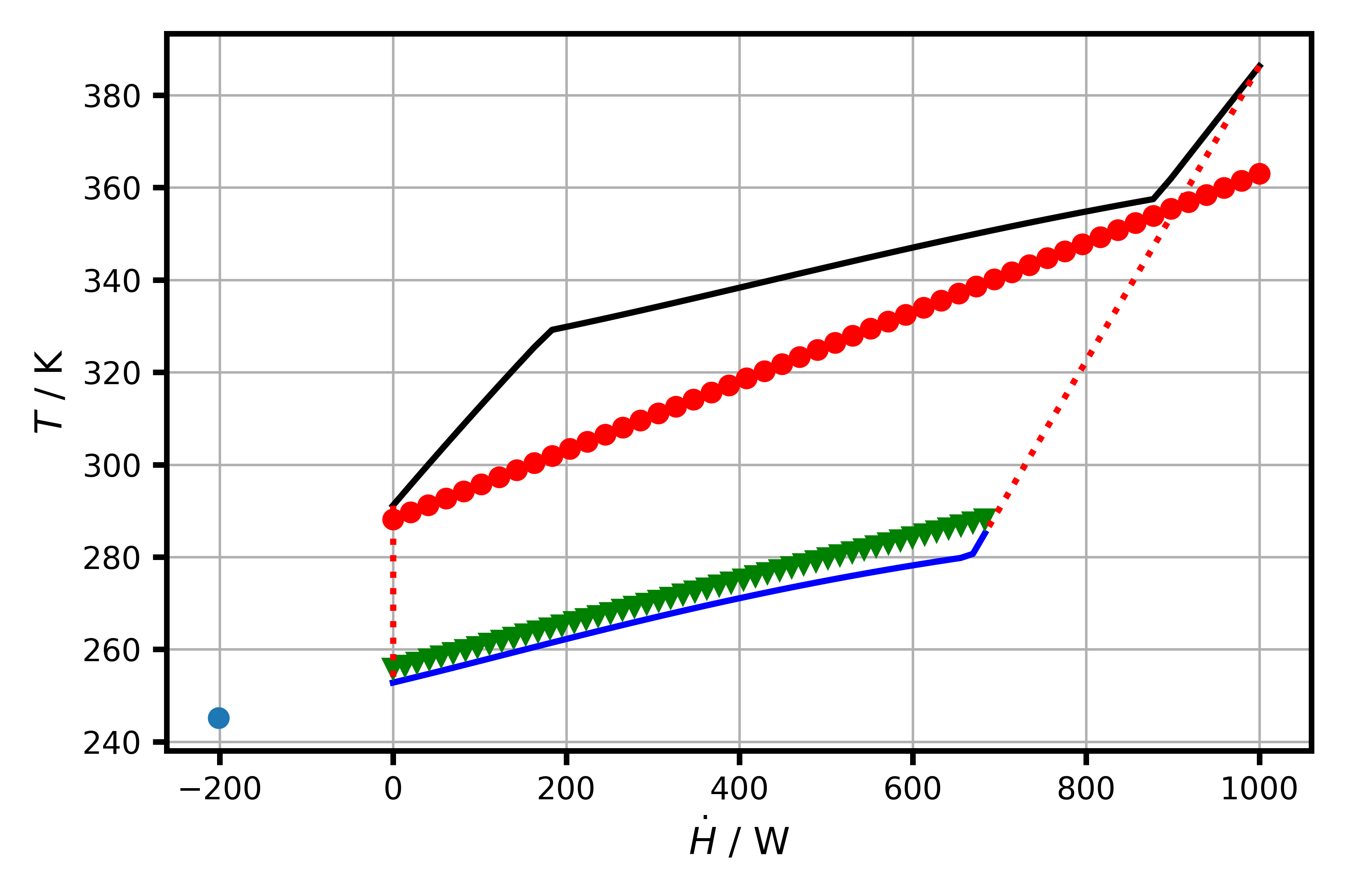
Heat Pump

For heat pumps of this simple structure (so far).

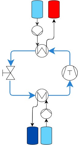
As one of the outputs, one gets such plots:

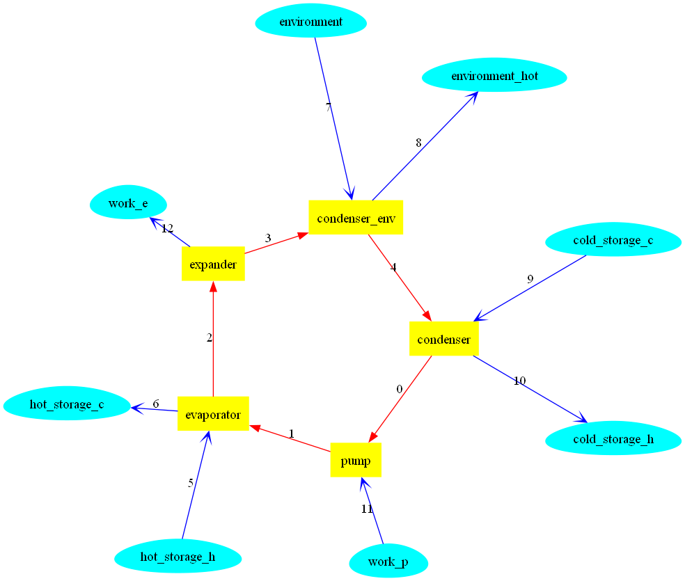
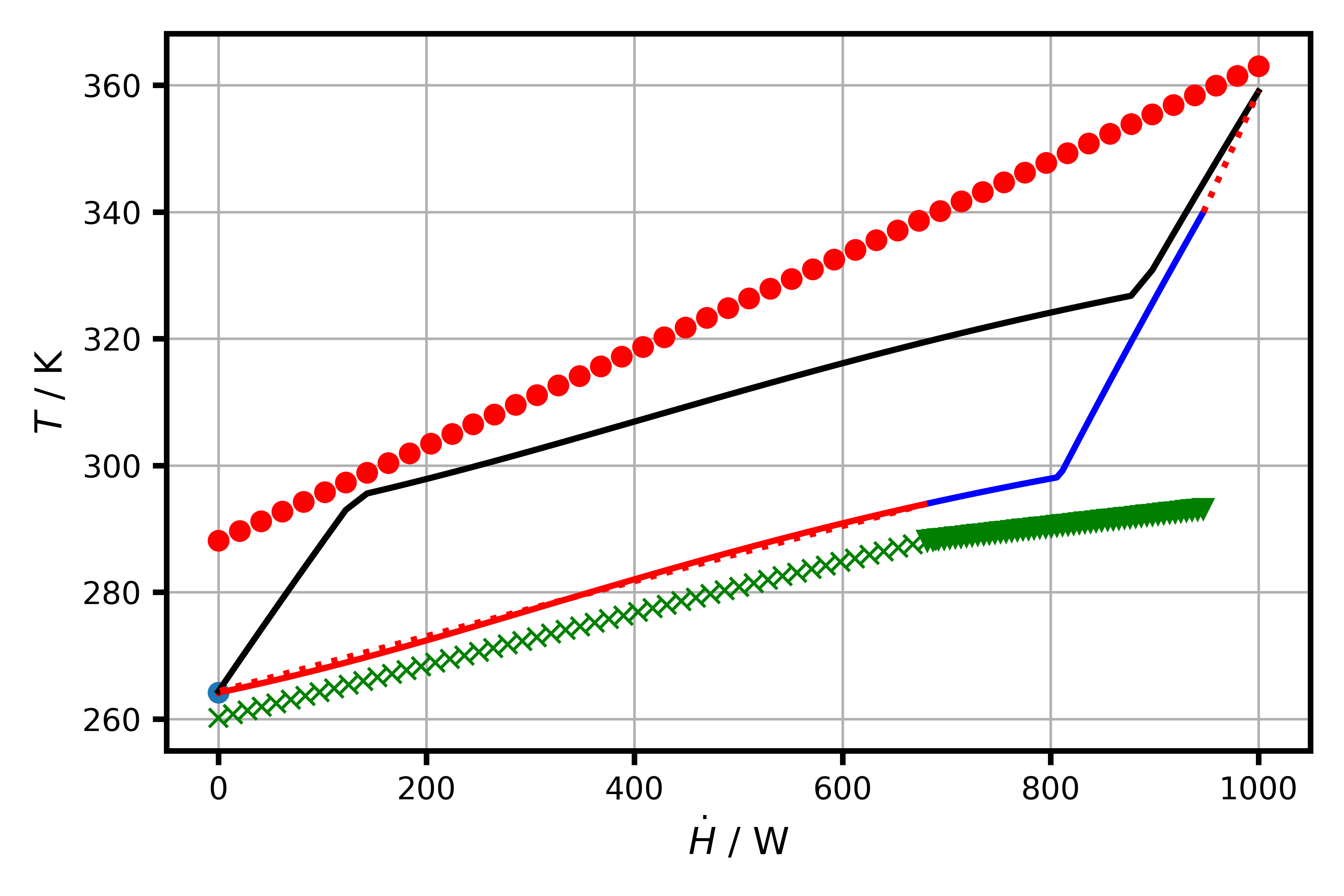
Organic Rankine Cycle

Organic Rankine cycles with this structure are modelled:

Typical results (here for a mixture) look like this:

Created on Sun May 21 10:52:09 2023

@author: atakan

class carbatpy.models.coupled.orc_simple_v2.OrganicRankineCycle(fluids, fixed_points, components=[])

Bases: object

Heat pump class for simple thermodynamic calculations for energy storage

Two pairwase storages at two different temperatures are assumed, always starting at room temperature (around 300K). Thus, three fluids are expected: the working fluid, the storage fluid or sink at high temperature (h) and the source storage fluid at low temperature. The minimum and maximum temperatures of all storags are fixed and the heat flow rate to the high-T storage are given. Also, isentropic efficiencies are fixed so far, but they should use a function later.

__init__(fluids, fixed_points, components=[])

Heat pump class for simple thermodynamic calculations for energy storage

storages at two different temperatures, always starting at room temperature (around 300K). The minimum and maximum temperatures aof all storags are fixed and the heat flow rate to the high-T storage are given. Also, isentropic efficiencies. The COP_charging is important to reach a steady state. At the moment you will have to look it up from the heat pump calculation. It is used to divide the energy transfered to the envoronment and to the low temperature storage. Example for:

fixed_points = {“eta_s”: _ETA_S_, # expander

“eta_s_p”: _ETA_S_P_, # pump “p_low”: p_low, “p_high”: p_high, “T_hh”: _STORAGE_T_IN_, “h_h_out_sec”: state_sec_out[2], “h_h_out_w”: state_out_evap[2], “h_l_out_cold”: state_cold_out[2], “h_l_out_w”: state_out_cond[2], “h_env_in”: state_env_in[2], “h_env_out”: state_env_out[2], “T_hl”: _STORAGE_T_OUT_, “T_lh”: _COLD_STORAGE_T_OUT_, “T_ll”: _COLD_STORAGE_T_IN_, # 256.0, “Q_dot_h”: _Q_DOT_MIN_, “d_temp_min”: _D_T_MIN_, “cop_charging”: _COP_CHARGING # needed to calculate Q_env_discharging }

Parameters:

• fluids (list of three Fluid) – working fluid, secondary fluid to store at high T, cold fluid to store at low T.

• fixed_points (Dictionary) – all the fixed points are summarized here, the isentropic efficiency, the lower pressure(evaporator), the high and low temperatures of the high temperature storages, the same for the low temperature storages(source), the heat to be transfered at high T, the minimum approach temperature.

• components (TYPE, optional) – DESCRIPTION. The default is [].

Return type:

None.

calc_orc(verbose=False)

calculate a simple organic rankine cycle (ORC)

working with two sensible storages (or source and sink). At the moment the machine model is just for a constant isentropic efficiency. The initial states are provided by the Fluid-instances. The pressures have to be selected carefully, they are not tested at the moment. For optimization, the pressure levels of the cycle could be used within a second script. Several parameters are fixed along a calculation, this is in the dictionary “self.fixed_points”.

Parameters:

verbose (Boolean, optional) – should values be printed? The deault is False

Returns:

eta_orc – thermal efficiency of ORC.

Return type:

flaot

hp_plot(f_name='/home/docs/checkouts/readthedocs.org/user_builds/carbatpy-010/checkouts/stable/docs\\\\tests\\\\test_files\\last_T_H_dot_plot_orc', fig_ax=[])

plots the heat pump cycle and stores it to the given file (name)

Parameters:

• f_name (string, optional) – where to write the results and the plot.

• fig_ax (list (length 2), optional) – instances with figure and axes to plot into. If Empty a new one will be generated. default =[]

Return type:

None.

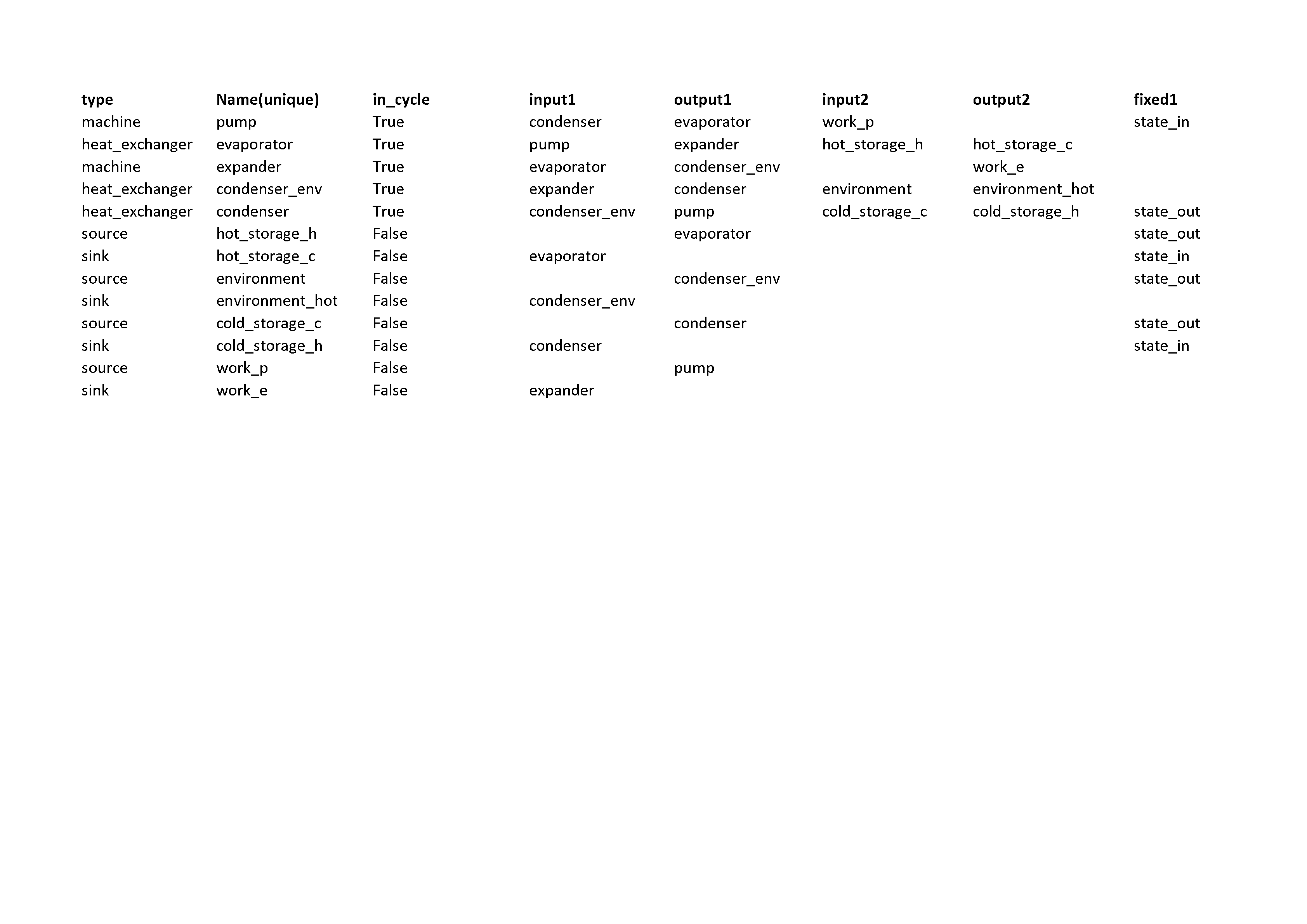
Cycle Structure

The structure of cycles are read from excel files , to create the structure plot, as shown above. graphviz must be installed on the computer to use this script. An exemplary excel-file is found in the data-folder. Here is the first page of it.

Created on Fri Dec 15 14:33:04 2023

@author: atakan

carbatpy.models.coupled.read_cycle_structure.plot_cycle_structure(fname, dirname='..//..//data', cycle_name='cycle', format_='png', engine='circo')

read an Excel file with information about the cycle structure and use graphviz

for visualization, a file is generated.

Parameters:

• fname (string) – the excel filename.

• dirname (string, optional) – the directory name to read the file and to store afterwards. The default is DIRNAME.

• cycle_name (string, optional) – name of the cycle. The default is “cyle”.

• format (String, optional) – plot-format (png, pdf etc). The default is “png”.

• engine (string, optional) – an engine name from graphviz (dot, circo etc.). The default is “circo”.

Return type:

None.